|
The algorithm derivation below can be found in Brierley [1] and Brierley and Batty [2]. Please refer to these for a hard copy.
This idea was first described by Werbos [3] and popularised by Rumelhart et al.[4].
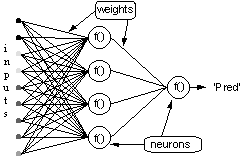
Fig 1 A multilayer perceptron
Consider the network above, with one layer of hidden neurons and one output neuron. When an input vector is propagated through the network, for the current set of weights there is an output Pred. The objective of supervised training is to adjust the weights so that the difference between the network output Pred and the required output Req is reduced. This requires an algorithm that reduces the absolute error, which is the same as reducing the squared error, where:
| Network Error | = | Pred - Req |
| = | E |
(1)
The algorithm should adjust the weights such that E2 is minimised. Back-propagation is such an algorithm that performs a gradient descent minimisation of E2.
In order to minimise E2, its sensitivity to each of the weights must be calculated. In other words, we need to know what effect changing each of the weights will have on E2. If this is known then the weights can be adjusted in the direction that reduces the absolute error.
The notation for the following description of the back-propagation rule is based on the diagram below.
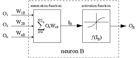
Fig 2 notation used
The dashed line represents a neuron B, which can be either a hidden or the output neuron. The outputs of n neurons (O
1
...O
n
) in the preceding layer provide the inputs to neuron B. If neuron B is in the hidden layer then this is simply the input vector.
These outputs are multiplied by the respective weights (W1B...WnB), where WnB is the weight connecting neuron n to neuron B. The summation function adds together all these products to provide the input, IB, that is processed by the activation function f (.) of neuron B. f (IB) is the output, OB, of neuron B.
For the purpose of this illustration, let neuron 1 be called neuron A and then consider the weight WAB connecting the two neurons.
The approximation used for the weight change is given by the delta rule:

(2)
where  is the learning rate parameter, which determines the rate of learning, and is the learning rate parameter, which determines the rate of learning, and

is the sensitivity of the error, E2, to the weight WAB and determines the direction of search in weight space for the new weight WAB(new) as illustrated in the figure below.
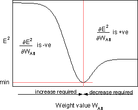
Fig 3 In order to minimise E2 the delta rule gives the direction of weight change required
From the chain rule,

(3)
and
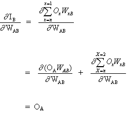
(4)
since the rest of the inputs to neuron B have no dependency on the weight WAB.
Thus from eqns. (3) and (4), eqn. (2) becomes,

(5)
and the weight change of WAB depends on the sensitivity of the squared error, E2, to the input, IB, of unit B and on the input signal OA.
There are two possible situations:
1. B is the output neuron;
2. B is a hidden neuron.
Considering the first case:
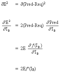
Since B is the output neuron, the change in the squared error due to an adjustment of WAB is simply the change in the squared error of the output of B:
(6)
combining eqn. (5) with (6) we get,

(7)
the rule for modifying the weights when neuron B is an output neuron.
If the output activation function, f (.), is the logistic function then:

(8)
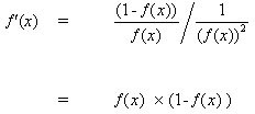
differentiating (8) by its argument x;

(9)
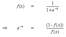
But,
(11)
inserting (11) into (9) gives:
(12)
similarly for the tanh function,

or for the linear (identity) function,

This gives:

Considering the second case:
B is a hidden neuron.

(13)
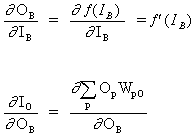
where the subscript, o, represents the output neuron.
(15)
where p is an index that ranges over all the neurons including neuron B that provide input signals to the output neuron. Expanding the right hand side of equation (15),

(16)
since the weights of the other neurons ,WpO (p!=B) have no dependency on OB.
Inserting (14) and (16) into (13),

(17)
Thus  is now expressed as a function of is now expressed as a function of  , calculated as in (6). , calculated as in (6).
The complete rule for modifying the weight WAB between a neuron A sending a signal to a neuron B is,

(18)
where,
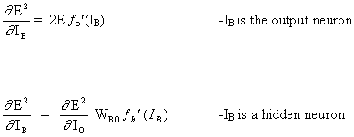
where fo(.) and fh(.)are the output and hidden activation functions respectively.
Example
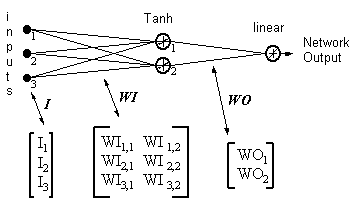
Network Output = [tanh(IT .WI)] . WO
let
HID = [Tanh(IT.WI)]T - the outputs of the hidden neurons
ERROR = (Network Output - Required Output)
LR = learning rate
The weight updates become,
linear output neuron
WO = WO - ( LR x ERROR x HID )
(21)
tanh hidden neuron
WI = WI - { LR x [ERROR x WO x (1- HID2)] . IT }T
(22)
Equations 21 and 22 show that the weight change is an input signal multiplied by a local gradient. This gives a direction that also has magnitude dependent on the magnitude of the error. If the direction is taken with no magnitude then all changes will be of equal size which will depend on the learning rate.
The algorithm above is a simplified version in that there is only one output neuron. In the original algorithm more than one output is allowed and the gradient descent minimises the total squared error of all the outputs. With only one output this reduces to minimising the error.
There are many algorithms that have evolved from the original algorithm with the aim to increase the learning speed. These are summarised in [5].
References
[1] P.Brierley, Appendix A in "Some Practical Applications of Neural Networks in the Electricity Industry" Eng.D. Thesis, 1998, Cranfield University, UK.
[2] P.Brierley and B.Batty, "Data mining with neural networks - an applied example in understanding electricity consumption patterns" in "Knowledge Discovery and Data Mining" (ed Max Bramer) 1999, chapter 12, pp.240-303, IEE, ISBN 0 85296 767 5.
[3] P.J. Werbos, "Beyond regression: New tools for prediction and analysis in the behavioural sciences," Ph.D. Thesis, 1974, Harvard University, Cambridge, MA.
[4] D.E. Rumelhart, G.E. Hinton and R.J. Williams, "Learning internal representation by error propagation," In Parallel Distributed Processing: Exploration in the Microstructure of Cognition (D.E Rumelhart and J.L. McClelland, eds.) 1986, vol. 1, chapter 8, Cambridge, MA, MIT Press.
[5] "Back Propagation family album" - Technical report C/TR96-05, Department of Computing, Macquarie University, NSW, Australia. www.comp.mq.edu.au/research.html
|